simple backtest

Numpy Simple Backtest

Numpyを使ったバックテスト

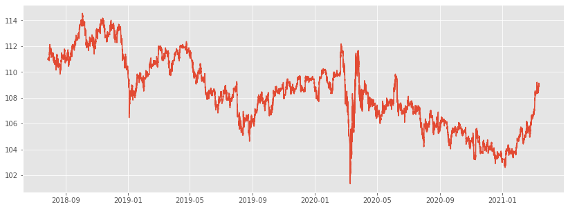
Numpy OHLCデータの読み込みとグラフ描画

(MT4 保存 15分足)

#   numpy等のインポート --------------------------------------------------------
import numpy as np
import time
import datetime

#   matplotlibのインポートと設定 ---------------------------------------------
import matplotlib.pyplot as plt
from pylab import rcParams # matplotlibの設定
rcParams['figure.figsize'] = 14,5 # 図のサイズ設定
plt.style.use('ggplot') # 色スタイル設定

#   csvデータの読み込み ------------------------------------------------------
"""
[['2018.07.20' '21:30' '111.477' '111.518' '111.462' '111.467' '827']
 ['2018.07.20' '21:45' '111.467' '111.479' '111.381' '111.444' '470']
 ['2018.07.22' '22:00' '111.364' '111.432' '111.363' '111.419' '107']]
"""
data = np.loadtxt("USDJPY15.csv",delimiter=",", dtype='str') # 文字列として読み込み

#   文字列データの日付datetimeへの変換と、float数値への変換
data = [[ datetime.datetime.fromisoformat("-".join((i[0]+" "+i[1]).split(".")))
         , float(i[2]), float(i[3]), float(i[4]), float(i[5]), float(i[6])] for i in data]
#data = [i for i in data if i[0] > datetime.datetime.fromisoformat('2019-01-01 00:00') ]

#   Close価格のグラフ化 ------------------------------------------------------
x = [i[0] for i in data]
y = [i[4] for i in data]
plt.plot(x, y)
#plt.savefig("figure1.png")
plt.show()

Numpy シンプルバックテスト

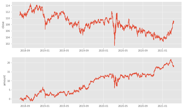
#   バックテスト -------------------------------------------------------------
lot = 1 # 売買ロット
position = 0 # 保有ポジション
amount_start = 0 # 初期証拠金
amount = amount_start # 証拠金残高
profit_y = [] # 資産推移
close = np.array([]) # 終値
count = 0 #売買カウント

for tick in data:
    now = tick[0]
    ltp = tick[4] # last traded price
    profit_y.append( amount + (position*ltp*lot) ) # 資産推移

    close = np.append(close,ltp)
    close = close[-1000:]

    if len(close) < 1000:
        pass

    smaA = np.mean(close[-1000:])
    smaB = np.mean(close[-400:])

    if smaA > smaB and position < 1:
        "BUY"
        if position < 0: # 保有ポジション決済
            amount = amount - ltp*lot
            position += 1
        amount = amount - ltp*lot # 買注文
        position += 1 # ポジション保有数
        count += 1

    elif smaA < smaB and position > -1:
        "SELL"
        if position > 0: # 保有ポジション決済
            amount = amount + ltp*lot
            position -= 1
        amount = amount + ltp*lot # 売注文
        position -= 1 # ポジション保有数
        count += 1

amount_all = amount + (position*ltp*lot) # 取引後資産
profit = amount_all - count * lot * 0.012 # スプレッド分差し引き

print("取引回数(簡易):", count)
print("開始時資産 :",amount_start)
print("獲得値幅 :",round(amount_all,5))
print("利益 :",round(profit,5))

取引回数(簡易): 87
開始時資産 : 0
獲得値幅 : 17.799
利益 : 16.755

x = [i[0] for i in data]
y = [i[4] for i in data]

import matplotlib.pyplot as plt
plt.style.use("ggplot")
fig = plt.figure(figsize=(13,8))

#   Close価格のグラフ化 ------------------------------------------------------
ax1 = fig.add_subplot(211)
ax1.set_ylabel("close")
ax1.plot(x, y)

#   資産変動のグラフ化 -------------------------------------------------------
ax2 = fig.add_subplot(212)
ax2.set_ylabel("amount") 
ax2.plot(x, profit_y)

#plt.savefig("figure2.png")
plt.show()

---

---

Pandas Simple Backtest

Pandasを使ったバックテスト

Pandas OHLCデータの読み込みとグラフ描画

(MT4 保存 15分足)

import pandas as pd
import datetime

"""
# USDJPY15.csv
2018.07.20,21:30,111.477,111.518,111.462,111.467,827
2018.07.20,21:45,111.467,111.479,111.381,111.444,470
2018.07.22,22:00,111.364,111.432,111.363,111.419,107
"""
df_ohlc = pd.read_csv("USDJPY15.csv", header=None)
df_ohlc[0] = df_ohlc[0] +" "+ df_ohlc[1]
df_ohlc[0] = pd.to_datetime(df_ohlc[0])
df_ohlc.columns = ["date","time","open","high","low","close","volume"]
df_ohlc.index = df_ohlc["date"]
del df_ohlc["time"]
del df_ohlc["date"]
df_ohlc[["close"]].plot()
df_ohlc.head(5)

Pandas シンプルバックテスト

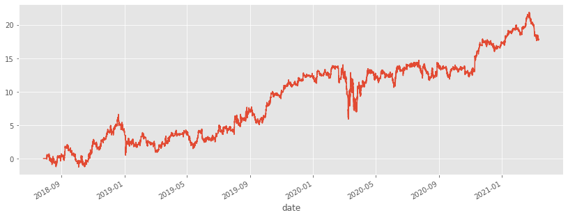
Pandasを使ったバックテスト

df = df_ohlc.copy()
df = df[datetime.datetime(2018,1,1):]

df["smaA"] = df["close"].rolling(window=400,min_periods=1).mean()
df["smaB"] = df["close"].rolling(window=1000,min_periods=1).mean()

df["signal"] = 0
df.loc[ df["smaA"] < df["smaB"] ,"signal"] = 1
df.loc[ df["smaA"] > df["smaB"] ,"signal"] = -1

count = df['signal'].diff().value_counts()
df['returns'] = df['close']-df['close'].shift(1)
df['strategy'] = df['returns'] * df['signal'].shift(1)
df['strategy'].cumsum().plot()

print("取引回数(簡易):",count.sum() - count[0])
v = df['strategy'].cumsum()[-1]
print("獲得値幅:",round(v,5))
profit = v - (count.sum() - count[0]) * 0.012
print("手数料差し引き後利益:",round(profit,5))

コードライセンスは CC0 もしくは Unlicense
Creative Commons — CC0 1.0 Universal
Unlicense.org » Unlicense Yourself: Set Your Code Free